Skip to content

Stress distribution under loads

The classical elastic solutions for stress beneath surface loads — Boussinesq (1885), Westergaard (1938), Newmark / Fadum (1935, 1948) — plus the 2:1 empirical approximation used in everyday practice.

Quick examples

Python
import geoeq as ge

# Concentrated point load
ge.boussinesq_point(P=100, z=2, r=0)             # 11.94 kPa under the load
ge.boussinesq_point(P=100, z=2, r=3)             # 0.66 kPa, off-axis

# Infinite line load (kN per m of line)
ge.boussinesq_line(q=50, z=3, x=0)

# Uniformly loaded strip of width B
ge.boussinesq_strip(q=100, B=2, z=1, x=0)

# Centreline stress under a uniformly loaded circle
ge.boussinesq_circular(q=100, R=2, z=2)          # 64.65 kPa — matches Das Table 6.6

# Rectangle B x L (Newmark/Fadum via corner influence)
ge.boussinesq_rect(q=100, B=4, L=6, z=2, position="centre")

Newmark / Fadum influence value

For a corner of a \(B \times L\) rectangle at depth \(z\), with \(m = B/z\) and \(n = L/z\):

\[ \begin{aligned} I = \frac{1}{4\pi}\Bigg\{ & \frac{2mn\sqrt{m^2 + n^2 + 1}}{m^2 + n^2 + m^2 n^2 + 1} \cdot \frac{m^2 + n^2 + 2}{m^2 + n^2 + 1} \\ & + \tan^{-1}\!\Bigg[\frac{2mn\sqrt{m^2+n^2+1}}{m^2+n^2-m^2n^2+1}\Bigg] \Bigg\} \end{aligned} \]
Python
ge.newmark_influence(m=1.0, n=1.0)   # 0.1752 — matches Das Table 6.5

Stress under the centre of a rectangle is then computed by superposition of four corner-rectangles each of size \((B/2) \times (L/2)\).

Pressure bulb

The "pressure bulb" — the locus of points carrying a given percentage of the surface stress — is the picture textbooks use to explain why footings need to consider deep soil:
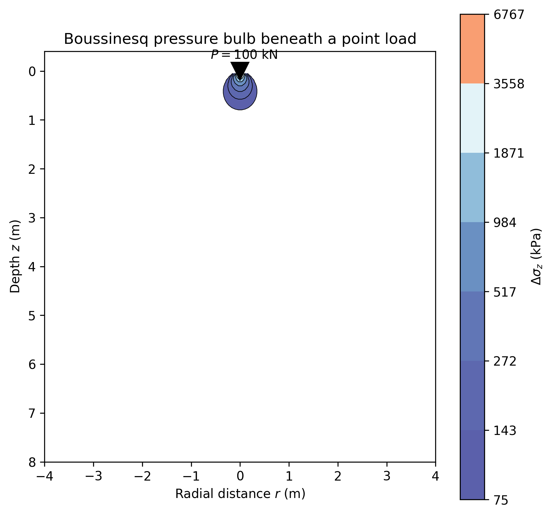
Pressure bulb

Boussinesq pressure bulb under a 100 kN point load. Generated by ge.stress_isobar_plot().

Westergaard for stratified media

When alternating thin stiff/soft layers prevent lateral straining, Westergaard's solution is more appropriate than Boussinesq:

\[ \Delta\sigma_z = \frac{P}{\pi z^2}\cdot \frac{\eta}{[\eta^2 + (r/z)^2]^{3/2}}, \quad \eta = \sqrt{\frac{1 - 2\mu}{2 - 2\mu}}. \]
Python
ge.westergaard_point(P=100, z=2, r=0, mu=0.0)

2:1 approximation

The 2:1 spread is empirical but widely used for spread footings up to \(z \approx 2B\):

\[ \Delta\sigma_z = \frac{q\,B\,L}{(B + z)(L + z)} \]
Python
ge.stress_2to1(q=100, B=2, L=4, z=5)             # 12.70 kPa

API reference

boussinesq_point

Python
boussinesq_point(P: float, z: float, r: float = 0.0) -> float

Vertical stress under a point load on a semi-infinite elastic mass.

Text Only
delta_sigma_z = (3 P / (2 pi z^2)) * (1 / (1 + (r/z)^2))^(5/2)
PARAMETER DESCRIPTION
P

Point load (kN).

TYPE: float

z

Depth below ground surface (m).

TYPE: float

r

Radial distance from the line of action (m).

TYPE: float DEFAULT: 0.0

RETURNS DESCRIPTION
delta_sigma

Vertical stress increment (kPa).

TYPE: float

Reference

Boussinesq (1885); Das (2010) Eq. 6.4.

Source code in geoeq/design/boussinesq.py
Python
def boussinesq_point(P: float, z: float, r: float = 0.0) -> float:
    """Vertical stress under a point load on a semi-infinite elastic mass.

        delta_sigma_z = (3 P / (2 pi z^2)) * (1 / (1 + (r/z)^2))^(5/2)

    Parameters
    ----------
    P : float
        Point load (kN).
    z : float
        Depth below ground surface (m).
    r : float
        Radial distance from the line of action (m).

    Returns
    -------
    delta_sigma : float
        Vertical stress increment (kPa).

    Reference
    ---------
    Boussinesq (1885); Das (2010) Eq. 6.4.
    """
    check_positive(z, "z")
    check_non_negative(r, "r")
    ratio = 1.0 / (1.0 + (r / z) ** 2)
    return float(3 * P / (2 * np.pi * z ** 2) * ratio ** 2.5)

boussinesq_line

Python
boussinesq_line(q: float, z: float, x: float = 0.0) -> float

Vertical stress under an infinite line load q (kN/m).

Text Only
delta_sigma_z = (2 q / pi z) * 1 / (1 + (x/z)^2)^2
Reference

Das (2010) Eq. 6.7.

Source code in geoeq/design/boussinesq.py
Python
def boussinesq_line(q: float, z: float, x: float = 0.0) -> float:
    """Vertical stress under an infinite line load q (kN/m).

        delta_sigma_z = (2 q / pi z) * 1 / (1 + (x/z)^2)^2

    Reference
    ---------
    Das (2010) Eq. 6.7.
    """
    check_positive(z, "z")
    return float(2 * q / (np.pi * z) * 1 / (1 + (x / z) ** 2) ** 2)

boussinesq_strip

Python
boussinesq_strip(q: float, B: float, z: float, x: float = 0.0) -> float

Vertical stress under a uniformly loaded infinite strip of width B.

Text Only
delta_sigma_z = (q / pi) * [ alpha + sin(alpha) cos(alpha + 2 beta) ]

where alpha and beta are the angles subtended at the point by the edges of the strip (Das Eq. 6.10).

PARAMETER DESCRIPTION
q

Surface pressure (kPa).

TYPE: float

B

Strip width (m).

TYPE: float

z

Depth (m).

TYPE: float

x

Horizontal distance from the centre of the strip (m).

TYPE: float DEFAULT: 0.0

Reference

Das (2010) Eq. 6.10.

Source code in geoeq/design/boussinesq.py
Python
def boussinesq_strip(q: float, B: float, z: float, x: float = 0.0) -> float:
    """Vertical stress under a uniformly loaded infinite strip of width B.

        delta_sigma_z = (q / pi) * [ alpha + sin(alpha) cos(alpha + 2 beta) ]

    where alpha and beta are the angles subtended at the point by the
    edges of the strip (Das Eq. 6.10).

    Parameters
    ----------
    q : float
        Surface pressure (kPa).
    B : float
        Strip width (m).
    z : float
        Depth (m).
    x : float
        Horizontal distance from the *centre* of the strip (m).

    Reference
    ---------
    Das (2010) Eq. 6.10.
    """
    check_positive(z, "z")
    check_positive(B, "B")
    # Geometry: edges at x - B/2 and x + B/2, both at depth z.
    x1 = x - B / 2.0
    x2 = x + B / 2.0
    alpha = np.arctan(x2 / z) - np.arctan(x1 / z)
    # beta is the angle to the closer edge from the vertical (Das defn).
    beta = np.arctan(x1 / z)
    return float(q / np.pi * (alpha + np.sin(alpha) * np.cos(alpha + 2 * beta)))

boussinesq_circular

Python
boussinesq_circular(q: float, R: float, z: float) -> float

Vertical stress on the centreline beneath a uniformly loaded circle.

Text Only
delta_sigma_z = q * [ 1 - 1 / (1 + (R/z)^2)^(3/2) ]
Reference

Das (2010) Eq. 6.15.

Source code in geoeq/design/boussinesq.py
Python
def boussinesq_circular(q: float, R: float, z: float) -> float:
    """Vertical stress on the centreline beneath a uniformly loaded circle.

        delta_sigma_z = q * [ 1 - 1 / (1 + (R/z)^2)^(3/2) ]

    Reference
    ---------
    Das (2010) Eq. 6.15.
    """
    check_positive(z, "z")
    check_positive(R, "R")
    return float(q * (1 - 1 / (1 + (R / z) ** 2) ** 1.5))

newmark_influence

Python
newmark_influence(m: float, n: float) -> float

Fadum / Newmark influence value I for a rectangle B x L at depth z.

Text Only
m = B / z,   n = L / z
RETURNS DESCRIPTION
I

Dimensionless influence factor (Das Eq. 6.30). The stress at the corner of a uniformly loaded B x L rectangle is q * I.

TYPE: float

Reference

Fadum (1948); Newmark (1935); Das Eq. 6.30, Table 6.5.

Source code in geoeq/design/boussinesq.py
Python
def newmark_influence(m: float, n: float) -> float:
    """Fadum / Newmark influence value I for a rectangle B x L at depth z.

        m = B / z,   n = L / z

    Returns
    -------
    I : float
        Dimensionless influence factor (Das Eq. 6.30). The stress at the
        corner of a uniformly loaded B x L rectangle is q * I.

    Reference
    ---------
    Fadum (1948); Newmark (1935); Das Eq. 6.30, Table 6.5.
    """
    check_positive(m, "m")
    check_positive(n, "n")
    # Fadum's closed-form.
    s = m * m + n * n + 1.0
    term1 = (2 * m * n * np.sqrt(s)) / (s + m * m * n * n) * (s + 1) / s
    # Newmark formula (Fadum 1948):
    # I = (1/4 pi) * { 2 m n sqrt(m^2+n^2+1) / (m^2+n^2+1 + m^2 n^2)
    #                  * (m^2+n^2+2)/(m^2+n^2+1)
    #                 + atan( 2 m n sqrt(m^2+n^2+1) / (m^2+n^2+1 - m^2 n^2) ) }
    a = 2 * m * n * np.sqrt(s)
    b = s + m * m * n * n
    c = (s + 1) / s
    d = s - m * m * n * n
    atan_arg = a / d
    # When d < 0, the angle is in the second quadrant and we add pi.
    if d > 0:
        atan_term = np.arctan(atan_arg)
    else:
        atan_term = np.arctan(atan_arg) + np.pi
    I = (1.0 / (4 * np.pi)) * (a / b * c + atan_term)
    return float(I)

boussinesq_rect

Python
boussinesq_rect(q: float, B: float, L: float, z: float, position: str = 'corner') -> float

Vertical stress under a uniformly loaded rectangle B x L.

Uses Fadum (1948) corner influence value, with superposition for 'centre' (4x mB/2 x L/2 sub-rectangles) and 'edge_mid' positions.

PARAMETER DESCRIPTION
q

Surface pressure (kPa).

TYPE: float

B

Rectangle dimensions (m). Convention: L >= B.

TYPE: float

L

Rectangle dimensions (m). Convention: L >= B.

TYPE: float

z

Depth below surface (m).

TYPE: float

position

'corner' -- under one corner of the rectangle 'centre' -- under the centre (sum of 4 sub-rectangles) 'edge' -- under the midpoint of a long edge (2 sub-rectangles)

TYPE: str DEFAULT: 'corner'

Reference

Fadum (1948); Das (2010) Eq. 6.29-6.31.

Source code in geoeq/design/boussinesq.py
Python
def boussinesq_rect(
    q: float, B: float, L: float, z: float, position: str = "corner",
) -> float:
    """Vertical stress under a uniformly loaded rectangle B x L.

    Uses Fadum (1948) corner influence value, with superposition for
    'centre' (4x mB/2 x L/2 sub-rectangles) and 'edge_mid' positions.

    Parameters
    ----------
    q : float
        Surface pressure (kPa).
    B, L : float
        Rectangle dimensions (m). Convention: L >= B.
    z : float
        Depth below surface (m).
    position : str
        'corner'  -- under one corner of the rectangle
        'centre'  -- under the centre (sum of 4 sub-rectangles)
        'edge'    -- under the midpoint of a long edge (2 sub-rectangles)

    Reference
    ---------
    Fadum (1948); Das (2010) Eq. 6.29-6.31.
    """
    check_positive(z, "z")
    check_positive(B, "B")
    check_positive(L, "L")
    position = position.lower()

    if position == "corner":
        I = newmark_influence(B / z, L / z)
        return float(q * I)
    elif position in ("centre", "center"):
        # Four rectangles each B/2 x L/2 sharing a corner at the centre.
        I = newmark_influence((B / 2) / z, (L / 2) / z)
        return float(q * 4 * I)
    elif position == "edge":
        # Two rectangles each B/2 x L sharing a corner at the edge mid.
        I = newmark_influence((B / 2) / z, L / z)
        return float(q * 2 * I)
    raise ValueError("position must be 'corner', 'centre', or 'edge'.")

westergaard_point

Python
westergaard_point(P: float, z: float, r: float = 0.0, mu: float = 0.0) -> float

Westergaard vertical stress for a point load on a layered medium.

Text Only
delta_sigma_z = (P / (pi z^2)) * eta / (eta^2 + (r/z)^2)^(3/2)

where eta = sqrt( (1 - 2mu) / (2 - 2mu) ).

For thinly stratified soils (alternating stiff/soft) the Westergaard solution gives lower stresses than Boussinesq.

Reference

Westergaard (1938); Das (2010) Eq. 6.13.

Source code in geoeq/design/boussinesq.py
Python
def westergaard_point(P: float, z: float, r: float = 0.0, mu: float = 0.0) -> float:
    """Westergaard vertical stress for a point load on a layered medium.

        delta_sigma_z = (P / (pi z^2)) * eta / (eta^2 + (r/z)^2)^(3/2)

    where eta = sqrt( (1 - 2mu) / (2 - 2mu) ).

    For thinly stratified soils (alternating stiff/soft) the Westergaard
    solution gives lower stresses than Boussinesq.

    Reference
    ---------
    Westergaard (1938); Das (2010) Eq. 6.13.
    """
    check_positive(z, "z")
    check_non_negative(r, "r")
    if not 0 <= mu < 0.5:
        raise ValueError("mu must be in [0, 0.5).")
    eta_sq = (1 - 2 * mu) / (2 - 2 * mu) if mu < 0.5 else 0.0
    eta = np.sqrt(eta_sq) if eta_sq > 0 else 1e-9
    return float(P / (np.pi * z ** 2) * eta / (eta_sq + (r / z) ** 2) ** 1.5)

stress_2to1

Python
stress_2to1(q: float, B: float, L: float, z: float) -> float

2:1 vertical-spread approximation for a B x L footing.

Text Only
delta_sigma_z = q * B * L / ((B + z) * (L + z))

Crude but engineering-useful for spread footings up to z ~ 2B.

Reference

Das (2010) Eq. 6.34.

Source code in geoeq/design/boussinesq.py
Python
def stress_2to1(q: float, B: float, L: float, z: float) -> float:
    """2:1 vertical-spread approximation for a B x L footing.

        delta_sigma_z = q * B * L / ((B + z) * (L + z))

    Crude but engineering-useful for spread footings up to z ~ 2B.

    Reference
    ---------
    Das (2010) Eq. 6.34.
    """
    check_positive(z, "z")
    check_positive(B, "B")
    check_positive(L, "L")
    return float(q * B * L / ((B + z) * (L + z)))

stress_bulb

Python
stress_bulb(P: float, z_range=None, r_range=None, n: int = 50)

Compute a stress-bulb mesh under a point load.

RETURNS DESCRIPTION
dict with keys 'z', 'r', 'sigma' -- 2D grids suitable for contourf.
Reference

Das (2010) Fig. 6.6 (qualitative isobar pattern).

Source code in geoeq/design/boussinesq.py
Python
def stress_bulb(P: float, z_range=None, r_range=None, n: int = 50):
    """Compute a stress-bulb mesh under a point load.

    Returns
    -------
    dict with keys 'z', 'r', 'sigma' -- 2D grids suitable for contourf.

    Reference
    ---------
    Das (2010) Fig. 6.6 (qualitative isobar pattern).
    """
    if z_range is None:
        z_range = (0.1, 10.0)
    if r_range is None:
        r_range = (-5.0, 5.0)
    z = np.linspace(z_range[0], z_range[1], n)
    r = np.linspace(r_range[0], r_range[1], n)
    R, Z = np.meshgrid(r, z)
    ratio = 1.0 / (1.0 + (R / Z) ** 2)
    sigma = 3 * P / (2 * np.pi * Z ** 2) * ratio ** 2.5
    return {"z": Z, "r": R, "sigma": sigma}

stress_isobar_plot

Python
stress_isobar_plot(P: float = 100.0, z_max: float = 8.0, r_max: float = 4.0, levels=None, ax=None, save_as: str = None)

Stress isobars (pressure bulb) beneath a point load.

PARAMETER DESCRIPTION
P

Point load (kN).

TYPE: float DEFAULT: 100.0

z_max

Plot extents (m).

TYPE: float DEFAULT: 8.0

r_max

Plot extents (m).

TYPE: float DEFAULT: 8.0

levels

Iso-stress contour levels (kPa).

TYPE: sequence DEFAULT: None

Source code in geoeq/design/plots.py
Python
def stress_isobar_plot(P: float = 100.0, z_max: float = 8.0,
                       r_max: float = 4.0, levels=None,
                       ax=None, save_as: str = None):
    """Stress isobars (pressure bulb) beneath a point load.

    Parameters
    ----------
    P : float
        Point load (kN).
    z_max, r_max : float
        Plot extents (m).
    levels : sequence
        Iso-stress contour levels (kPa).
    """
    import matplotlib.pyplot as plt
    res = stress_bulb(P=P, z_range=(0.05, z_max),
                       r_range=(-r_max, r_max), n=120)
    if levels is None:
        # Geometric spacing from max stress in the grid.
        smax = np.nanmax(res["sigma"])
        levels = np.geomspace(max(smax * 0.01, 0.1), smax * 0.9, 8)
    if ax is None:
        fig, ax = plt.subplots(figsize=(7, 7))
    else:
        fig = ax.figure
    cs = ax.contourf(res["r"], res["z"], res["sigma"],
                     levels=levels, cmap="RdYlBu_r", alpha=0.8)
    ax.contour(res["r"], res["z"], res["sigma"],
               levels=levels, colors="black", linewidths=0.5)
    cbar = fig.colorbar(cs, ax=ax, label=r"$\Delta\sigma_z$ (kPa)")
    # Mark the load application point.
    ax.plot([0], [0], "v", color="black", markersize=14)
    ax.text(0, -0.2, f"  $P = {P:.0f}$ kN", ha="center", va="bottom",
            fontsize=10)
    ax.invert_yaxis()
    ax.set_xlabel(r"Radial distance $r$ (m)")
    ax.set_ylabel(r"Depth $z$ (m)")
    ax.set_title("Boussinesq pressure bulb beneath a point load")
    ax.set_aspect("equal")
    if save_as:
        fig.savefig(save_as, dpi=300, bbox_inches="tight")
    return fig